A Student's Guide to Cost-Benefit Analysis
Lesson 7 - Economic Theory Behind Cost and Benefit Valuation
Introduction
In order to conduct an economic CBA, you need to know:
1) cost of project inputs, and
2) the value of benefits
At first glance this may seem like a simple problem to solve:
1) total cost = number of input units x their purchase price, and
2) total benefits = units of output x their market selling price.
This approach is generally permissible for a private sector financial CBA, but not for a public sector economic CBA. The public sector economic CBA requires a broader definitions of costs and benefits that may differ in some instance from private financial CBA.
Valuing Project Costs
The costs of a project are related to the project inputs. Inputs are generally classified as: land, labor and capital.
The principle concept to keep in mind regarding input costs, is that, for CBA inputs must be priced at their social opportunity cost .
Social opportunity cost - the value that society must forego to use the input in the project; the value of the input’s best alternative use.
Does budgetary outlay ever equal social opportunity cost?
Boardman et al say, in most cases the answer is yes: budgetary outlay will equal opportunity cost (p. 67).
However, situations where divergence between budgetary outlay and opportunity cost can occur:
1) if the market for the input has inefficiencies
2) and/or the quantity of input demanded for the project is large relative to the total input market demand.
Boardman et al examine 3 situations:
1) There are no inefficiencies in the market for the input. They conclude:
budgetary outlay = opportunity cost.
2) There are no inefficiencies, but the project demands a large share of the market output thus generating noticeable price effects on the rest of society. Example: a dam that requires a lot of concrete thus bidding up regional concrete prices.
Conclude: budgetary outlay will diverge slightly from opportunity cost.
3) There are inefficiencies (failures) in the input market.
Concludes: budgetary outlay can diverge substantially from opportunity cost.
Boardman et al explore 3 examples of inefficient market, but say there can be hundreds of real-world examples.
Summary conclusions regarding costing of inputs:
1) Be especially alert to situations where the input market may have inefficient markets.
2) Follow these two rules:
Rule 1: True social opportunity cost = direct expenditure minus gains occurring in inefficient input markets
Rule 2: True social opportunity cost = direct expenditure plus losses occurring in inefficient input markets.
Valuing Project Benefits: Basic Welfare Economics
The valuation of project economic benefits requires some knowledge of welfare economics. The purpose of welfare economics is to measure changes (i.e., increase/decreases) in social welfare resulting from changes in economic conditions. Social welfare measures require an ability to measure changes in personal utility; i.e., changes in satisfaction that arise from changes in prices, and shifts in supply and demand schedules. In order to measure welfare impacts, we must look at:
1. Producers - the economic well-being of economic producers is measured by their net benefits (profits + fixed costs). This measure, the area under the price line and over the supply curve, has not been much disputed.
2. Consumers - measurement of the economic well-being of consumers, in contrast, has been fraught with academic controversy and difficulty. A brief history follows:
a. In 1844, French engineer Jules Dupuit develops the idea that the true measure of net benefits to consumers should be the enjoyment they receive in excess of the price they have to pay for the good; calls it consumers surplus.
b. In late 1800s, Alfred Marshall worked on money measures of utility change. He takes this, consumers surplus, to be the area under the demand curve and over the price line.
c. In 1940s Prof. J.R. Hicks establishes willingness-to-pay measures of consumer utility.
Hicks’ willingness-to-pay notion is formalized as compensating variation:
Explanation of compensating variation: Assume that an economic change (i.e., price change) does happen and it results in:
A welfare loss (i.e., due to a price increase) - then CV is the amount of money required as compensation to restore them to their pre-price-change level of utility.
A welfare gain (i.e., due to a price decrease) - then CV is the amount of money, if taken away from the person, would restore them to their pre-price-change level of utility.
Thus, money has been the basis of the 2 measures of consumer utility because personal utility cannot be measured directly. We have no happiness meter. Thus, an observable alternative (i.e., money) was chosen.
Welfare economics has largely chosen as its correct measure of consumer preferences willingness-to-pay; in other words, Hicks’ compensating variation. Because it restores individuals to their 'pre-price-change' level of utility.
But still, consumers surplus, along with producers surplus, are frequently used in applied welfare economics. Thus, we will explore CS & PS.
[Read: in Boardman et al App. 3A,p. 94, for a graphical comparison of CV & CS.]
Consumer Surplus and Compensating Variation
The aim of CBA & welfare economics is to measure the total impact of changes in price and demand resulting from government policy.
However, a measurement problem exists: an increase in Px will cause 2 types of economic losses:
a) substitution effect - a direct loss through the decrease in quantity demand of x due to change in Px
b) income effect - an indirect loss of income; the Δ in Px also Δ
=s the income you have to spend on other goods. If the consumer were to pay more for the good in question, her effective income would also be lowered.The aim of welfare economics is to measure both effects.
Problem with consumers surplus: it measures only the substitution effect.
The area under a regular (i.e., Marshallian) D-curve measures the substitution effect.
In contrast, a Hicksian (conceptual) demand curve:
a) includes the substitution effect (i.e., direct change in Dx due to change in Px)
b) also, includes (i.e., compensates for) the income effect
Thus, the area under a Hicksian D-curve exactly measures compensating variation; i.e., the full amount that it would take to restore an individual to his/her original level of utility given a price change.
CV is larger than CS because it compensates for the income effect as well as the substitution effect.
Thus the area under the Hicksian D-curves (CV) seems to be the correct measure of economic welfare.
Problem with Hicksian D-curves: they cannot be statistically estimated because...we cannot adjust for the income effect of price changes and thus hold utility constant.
Many economists (e.g., Samuelson) once said CS was a meaningless measure. Then came Willig (1976) and his "Consumers Surplus Without Apology." He concluded: The Δ CS resulting from a price ch
ange, is usually such a small fraction of total Y, that the income effect is negligible (i.e., usually the value of CS is within 95% of the value of CV).Hence, Consumers Surplus, rather than Compensating Variation, is frequently used without apology in CBA as a measure of consumer welfare.
Consumers and Producers Surpluses
1. Demand Curves:

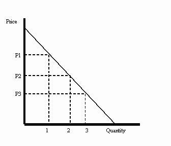
* X-axis represents the quantity of a good demanded at various prices
* Y axis represents the price paid for various quantities of the good
* the demand curve in negatively sloped due to the law of demand - q demanded is inversely related to price.
* the person would be willing-to-pay P1 for 1 unit, P2 for 2 units. etc.
The consumer will consume more units at a lower price than at a higher price.
This notion of the demand curve as a measure of willingness-to-pay is critical to the measurement of benefits for CBA.: Benefits are the sums of the maximum amounts people would be willing to pay in order to obtain outputs they view as desirable.
2. Measuring consumer gross and net benefits
How do we measure the benefit that an individual obtains from consumption?
* if a person pays P* for Q* units, we can thus infer from the graph that the gross value they place on consuming Q* is the area abcQ*. Thus we can say that:
gross benefits = the area under the demand curve (aka, total WTP).
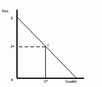
But this person has to pay something to consume this good. Cost of consumption = P*cQ*a. What are the net benefits?
net benefits = the area bcP*; or the area over the price line and below the demand curve.
Important concept:
Consumer surplus: This net benefits triangular area has a special name: consumer surplus = the area over the price line and below the demand curve. CS represents the excess of consumption enjoyment over the price paid.
Consumer surplus is an important concept in CBA and welfare economics because changes in consumer surplus provide reasonably correct estimates of the impacts of the benefits of consumers from government policies.
3. An Example of Consumer Welfare Impacts (Changes in CS)
Situation: Assume that the government institutes a policy (say a subsidy on consumption), that lowers the price of commodity x.
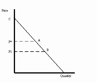
* P* falls to P1.
* consumption of x increases from x* to x1
Question: what happens to consumer welfare as measured by the change in consumers surplus?
Answer: consumer surplus increases by the amount equal to the area P*abP1.
Key: this sort of change in CS is taken to be the conceptually correct measure of the economic impacts of policy changes on consumers.
Computing the change in welfare:
a) as a trapezoid P1P*ab, or
b) as the difference in the area of the 2 triangles: cP1b - cP*a = P1P*ab
B. Economic Welfare of Producers
1. Supply curves
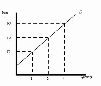
* axes, P & Q
* the supply curve represents the firm=s marginal variable cost of production
* the S curve slopes upward indicating that, at higher prices the firm will be willing to sell more units of x (P1-1 units, P2-2 units, P3-3 units)
* the area under the supply curve is the calculus integral of MC, i.e., TVC.
2. Measuring producer costs and profits
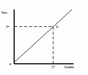
* assume that a firm faces a price of P*
* they will sell quantity Q*
* their total revenue; TR = P* x Q*
* and, if TVC is the area under the supply curve abQ*
* then the triangular area below the demand curve and over the supply curve (abP*) is a sort of profit + fixed cost
Important concept: Producers Surplus
* this profit + fixed cost is called producers surplus and this is the standard measure of the economic well-being of firms.
3. An Example of Producer Welfare Impacts (Changes in Producers Surplus)
Situation: Assume for some reason that price of commodity increases:
* price P1 rises to P2.
* production of x increases from x1 to x2
Question: what happens to producer welfare as measured by the change in producers surplus?
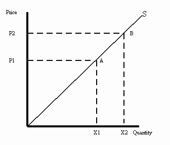
Answer: producer surplus increases by the amount equal to the trapezoidal area P2P1ab.
Key: this sort of change in PS is taken to be the appropriate measure of the economic impacts of policy changes on producers.
Computing the change in welfare, 2 ways:
a) as a trapezoid P1P2ab
b) as the difference in the area of the 2 triangles: cP2b - cP1a = P1P2ab
B. Summary of PS and CS
Producers and consumers surplus are the generally accepted measures of economic welfare.
It is the changes in PS and CS that ideally we want to estimate as measures of economic benefits from public policies. Changes in PS and CS measure the full impact of policy changes.
However, producers surplus has been better accepted than CS as a measure of economic well-being. CS is used in practice as benefits measure, but not without challenge.
Despite the controversy, CS remains the welfare measure of choice. (Willig’s paper said no problem changes in income and hence utility due to price change are so small as not to be an issue.)
Question: why can’t we simply use PxQ rather than CS as a measure of welfare impacts?
Answer: Because PxQ is simply the total amount paid for the good/service in question. PxQ ignores the gross WTP, the excess of enjoyment over price, and thus does not measure the full benefit received from the consumption of the good.
Valuing Welfare Impacts: Shifts in Supply & Demand Curves
We are now ready to examine conceptually correct measures of increases or decreases in benefits resulting from through shifts in the S & D curves. These are examples of the sort of economic welfare changes that public policies cause.
Key point: Benefit changes come through shifts in the S & D curves which, in turn, changes the size of the welfare triangles.
Examples of impacts:
Example #1 - stream improvement causes a demand curve shift for an angler, for graph see Loomis p.136.
Situation: an angler visits an unstocked stream several times a year to fish. The measure of WTP to fish is the cost of travel to the site (there is no admission fee).
Project: the state game and fish commission stocks the stream (at some cost of public funds). This improves the fishing success rate for the angler. This increases her WTP to visit the site.
Question: what are the benefits to this angler of the project?
Answer: the increase in consumers surplus due to the shift in the WTP curve.
Example #2 - range improvement cause a supply curve shift, for graph see Loomis p. 131.
Situation: a rancher grazes his cattle on public land. His cattle production is so small, he cannot effect the price of beef to consumers no matter how much he sells. He is a price-taker meaning the demand (WTP) curve is perfectly elastic (horizontal).
Project: BLM conducts a range improvement project (at some cost). They remove vegetation, add stock pond. This increases the carrying capacity of the land.
Question: what are the benefits to the rancher?
Answer: the increase in producers surplus due to a shift in his supply curve.
Welfare Impacts in Markets: A Project Potentially Affecting Both Consumers and Producers Market S & D curves - conceptually, are the horizontal summation of all individual S & D curves.
Example #3 - for graph see Loomis, p.134.
Situation: Consumers (households) and producers (i.e., industry) in a community rely on high-priced ground water.
Project: A public water supply project will provide reservoir water to a community to reduce its dependence on groundwater.
Question: what are the benefits to society (producers and consumers)?
Answer: The increase in CS + PS. Society as a whole benefits.
Distributional issues: Consumers gain, but producers fate is uncertain.
Links: